Group ICA with FSL’s Melodic
This guide will walk you through an independent components analysis of resting-state functional brain data using FSL’s Melodic tool. The type of ICA conducted in this guide is called multi-session temporal concatenation in the FSL documentation. This type of ICA will break down many participants resting-state scans into a set of common spatial and temporal components. I should mention that Melodic’s documentation is very nice. This guide is really a supplement to elaborate on the practicalities of running an ICA analysis and higher-level group analyses that are not discussed in FSL’s guide.
Disclaimer: I will attempt to explain the design choices I make, but you should thoroughly research all available options for your own analyses.
Disclaimer 2: I originally wrote this guide around 2014 and cannot guarantee it is up-to-date when you are reading it.
File Structure and Setup
I used Melodic version 3.14 from FSL build 506. All analyses were carried out on a cluster running Red Hat Enterprise Linux Server release 6.3 (Santiago). You should be working in an analysis directory with a structure similar to this one:
master_directory
├──   participants
│ ├──   001
│ │ ├──   001-functional.nii.gz
│ │ ├──   001-structural.nii.gz
│ │ └──   001-structural_brain.nii.gz
│ ├──   002
│ │ ├──   002-functional.nii.gz
│ │ ├──   002-structural.nii.gz
│ │ └──   002-structural_brain.nii.gz
│ └──   ...
├──   models
├──   designs
├──   presentation
└──   ev
    ├──   mean_translation.txt
    ├──   mean_rotation.txt
    └──   executive_function.txt
In this example, the functional images (e.g., 001-functional.nii.gz) were motion corrected with FSL. There are two structural images, the first is only oriented but not brain extracted because FSL’s new boundary-based registration (BBR) requires the skull be intact. The second structural is oriented and brain extracted (e.g., 001-structural_brain.nii.gz). Having both structural scans allows you to try different registration techniques, which I would recommend doing given how new BBR is to FSL’s default options. The models directory is where we will save Melodic’s .fsf configuration files (discussed below). The designs folder is where we will save our design matrices for higher-level group analyses (discussed in the Dual Regression section). The presentation folder is where we will store output images of ICA networks that can be used for presentations and manuscripts. Finally, the ev folder contains all of our behavioral data and control variables that we will use later to generate design matrices.
Configuring a Melodic Analysis
Here I will guide you through configuration of a Melodic analysis using the graphical user interface. Start the GUI with either melodic_gui or Melodic depending on your FSL install.
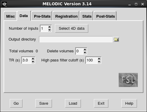
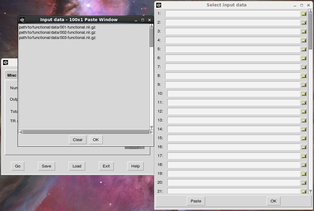
The first step in our configuration is to tell Melodic where to find the functional data. Set the number of inputs to your number of participants and click “Select 4D data”. Rather than browsing to each file separately (which would take a long time), we can just paste the file paths to your functionals. To generate a list of all the file paths, you can run a command like this:
$ find $PWD -name "*functional.nii.gz"
The find command will look for any file that ends in functional.nii.gz and print the full path as output to the terminal. For example:
path/to/functional/data/001-functional.nii.gz
path/to/functional/data/002-functional.nii.gz
...
path/to/functional/data/00n-functional.nii.gz
You can just select this list from the terminal output and paste it into the appropriate window:
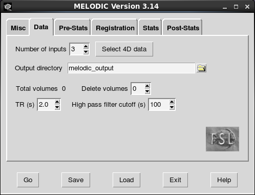
Next, name the output folder, the directory where you want your results to end up. I used “melodic_output” here, but you might want to use a more descriptive name in case you end up running multiple ICA analyses. Consider appending important preprocessing options to the output directory so it is easier to remember important differences between analyses. After you run the analysis, Melodic will create a directory with your specified name and the ending .gica (which stands for “group ica”, I think). In our case, a directory named “melodic_output.gica” will be created in the master_directory.
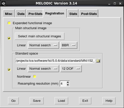
The next screen allows to you configure the registration steps. Boundary-based registration is the new default for registering participant’s functional scan to their structural scan. You can paste the paths to the structural scans using the same technique as above. BBR seems to be accurate and it is quite fast. However, you might want to try the 6 dof option as well. FSL makes it easy to switch back and forth between registration options. Paste in the file paths for the skull-stripped structural scans (the ones that end in “_brain”). If you switch to BBR, Melodic knows to look for the non-skull-stripped images in the same folder as the other structural image so long as there are no differences in the name other than “_brain”.
For standard space registration, the consensus option seems to be 12 dof. At this point, you can also choose the voxel size to do the analysis in. Melodic defaults to 4mm space as it saves compute time for some kinds of ICA (maybe all flavors of ICA). I leave it at the default, but you might want to run in 2mm or another voxel size. The pop-up window for the voxel size option says the added compute time is really only an issue for tensor ICA.
On the next screen, there are two important options: dimensionality estimation and ICA type. I would recommend leaving automatic dimensionality estimation on. If we are going through the trouble of utilizing a data-driven technique to derive resting-state network, you should probably avoid biasing the network creation step. For ICA type, you should change from the default of single-session ICA to multi-session temporal concatenation. Single subject ICA would be useful for denoising a single participant’s data. Tensor ICA is only useful if there is consistency among the participants’ experiences during the scan (e.g., they are all doing the same task). During resting-state, we do not have a common time course for the participants, so choose multi-session temporal concatenation. Please see the FSL documentation for usage scenarios for the different flavors of ICA.

On the final page, it is important to enable the full output of Melodic. The full output will give you a nifti image for each ICA component. Having those images makes it easier to generate figures for presentations/manuscripts.
The final configuration step is to save the configuration file. Click “Save” in the GUI, navigate to the models directory, and name the file something appropriately informative. The point of using the models directory is to prevent clutter in the master_directory.
Running Melodic
Starting the analysis is easy. Either hit “Go” in the GUI or exit the GUI and type:
$ feat models/melodic_analysis.fsf
Depending on your computing resources, Melodic can take a long time to run. For an analysis of 90 participants, Melodic takes ~20–30 minutes on a cluster running Xeon E5–2670 processors at 2.60GHz, ~45 minutes on an older cluster running Xeon E5540 processors at 2.53GHz, and ~6 hours on a 2011 4-core iMac.
Viewing Melodic ICA Components
After Melodic finishes, there are two ways to view the results. The first is to look at the components in the html report that is automatically generated by Melodic:
$ firefox melodic_output.gica/report.html
You can also explore the networks in more detail by looking at the actual 3D nifti images:
$ fslview melodic_output/bg_image.nii.gz melodic_output.gica/groupmelodic.ica/melodic_IC.nii.gz -l "Red-Yellow" -b 3,12
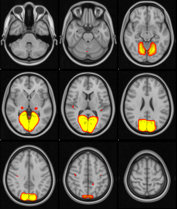
If you view melodic_IC.nii.gz, note that the networks are concatenated in the temporal dimension as if they are images acquired during different TRs. You can scroll through them by advancing through the volumes (red arrow in following image). Note also that the volumes/components start at 0 and not 1.

Compare Melodic ICA Components to Reference Networks
One popular technique for separating noise components from resting-state networks is to have an expert look at them and label networks as they see fit. In this section I will outline a more objective technique. Here we will use an FSL utility fslcc to spatially correlate all of our components to some set of reference networks. The reference networks I use are from a popular 7 network parcellation of cortex [1]. You can use any reference networks you want. Be sure the ones you choose are in the same space as your Melodic output. The reference networks should be concatenated in the temporal dimension with each volume corresponding to a different network. For the example below, I placed the reference networks into a new folder and named them with a descriptive name. The -t option lets you input an appropriate r-value threshold to determine if your component is significantly correlated with a reference networks. The output will only show you significantly similar networks this way.
$ fslcc --noabs -p 3 -t .204 reference_networks/yeo2011_7_liberal_combined_4mm.nii.gz melodic_output.gica/groupmelodic.ica/melodic_IC.nii.gz
The output looks like this:
  1   1 0.477
  1  12 0.478
  1  18 0.468
  2   6 0.473
  2  11 0.422
  2  24 0.439
  3  14 0.325
  3  17 0.498
  3  26 0.323
  4   4 0.410
  4  11 0.407
  4  14 0.228
  5  28 0.258
  6   4 0.271
  6   5 0.444
  6   9 0.285
  6  26 0.315
  7   9 0.232
  7  10 0.508
  7  15 0.502
The first column is the reference network number. A sample interpretation of the results (first three rows) is that there were three ICA components that significantly correlate with the first Yeo network (networks 1, 12, and 18). The first Yeo network is the visual network, so components 1, 12, and 18 are likely different parts of the visual system. In fact, the fslview screen shot above is of network 1, so we have some confirmation that visual regions are involved in this network.
One final check to ensure a component is a resting-state network is to verify that the bulk of the component’s signal falls on the lower end of the power frequency spectrum. Melodic a provides suitable figure for each component in the html report:
Rendering Images of ICA Networks
This section walks through the process of getting Melodic output ready for presentation. We’ve already looked at the networks in fslview, now we want to make some images of the networks at different levels for the purposes of a PowerPoint presentation or manuscript. The first step we want to take is to change Melodic’s output from 4mm space to a much higher resolution space. We can use flirt for that. The following command changes melodic output to 0.5mm space. You can go to any voxel size for which you have a reference image. If you want to go to a different voxel size, change the argument $FSLDIR/data/standard/MNI152_T1_0.5mm.nii.gz to reference another MNI template.
for i in {1..29}; do
    flirt -in melodic_output.gica/groupmelodic.ica/stats/thresh_zstat$i.nii.gz -ref $FSLDIR/data/standard/MNI152_T1_0.5mm -applyxfm -usesqform -out presentation/thresh_zstat${i}_highres.nii.gz
done
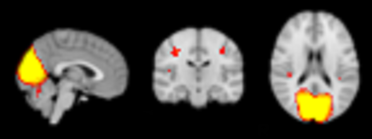
Low resolution output:
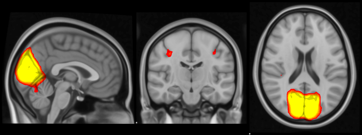
High resolution output:
The next step is to make image files of each network. Below I loop through every network and renders an image of the mid-sagittal, -coronal and -axial slices.
for i in {1..29}; do
    overlay 1 0 $FSLDIR/data/standard/MNI152_T1_0.5mm -A presentation/thresh_zstat${i}_highres.nii.gz 2.5 10 presentation/${i}_overlay.nii.gz
    slicer presentation/${i}_overlay.nii.gz -a presentation/${i}_sliced.ppm
    convert presentation/${i}_sliced.ppm presentation/${i}_sliced.png
done
An alternative to slicer’s -a option is -S 24 1200 which would render every 24th axial slice and re-size the final output to be less than 1200 pixels wide.
If you only care about one or two networks, you can just use the overlay and slicer commands on the network you are interested in. In this case, I was interested in making a report of all networks from my analysis, so the for loop is handy. My ICA yielded 29 components; if you have a different number of components, you will need to adjust the range in the curly brackets at the start of the for loop.
References
Yeo, B. T. T., Krienen, F. M., Sepulcre, J., Sabuncu, M. R., Lashkari, D., Hollinshead, M., … Buckner, R. L. (2011). The organization of the human cerebral cortex estimated by intrinsic functional connectivity. Journal of Neurophysiology, 106(3), 1125–65. doi:10.1152/jn.00338.2011