Dual Regression
Disclaimer: I originally wrote this guide around 2015 and cannot guarantee it is up-to-date when you are reading it.
This is the second part of my guide to running group analyses on resting-state brain data. In the first part, we generated some resting-state networks using FSL’s Melodic tool. Here I will discuss the practicalities of investigating spatial and intensity differences in those resting-state networks as a function of individual differences in some individual (e.g., intelligence) or group difference (e.g., patient vs. control). I will be using another FSL tool, dual regression, for this analysis.
I should note that this guide assumes you’ve used my ICA guide and have a similar directory structure to the one below:
master_directory
    ├──   participants
    │ ├──   001
    │ │ ├──   001-functional.nii.gz
    │ │ ├──   001-structural.nii.gz
    │ │ └──   001-structural_brain.nii.gz
    │ ├──   002
    │ │ ├──   002-functional.nii.gz
    │ │ ├──   002-structural.nii.gz
    │ │ └──   002-structural_brain.nii.gz
    │ └──   ...
    ├──   models
    ├──   designs
    ├──   presentation
    ├──   melodic_output.gica
    │ └──   groupmelodic.ica
    │     └──   melodic_IC.nii.gz
    ├──   reference networks
    │ └──   yeo2011_7_liberal_combined.nii.gz
    └──   ev
        ├──   mean_translation.txt
        ├──   mean_rotation.txt
        └──   executive_function.txt
Disclaimer: I will attempt to explain the design choices I make, but you should thoroughly research all available options for your own analyses.
Configuring Dual Regression
The first thing we need to do is set up a model for dual regression. This model is very similar to the design matrix you might use in a higher level model. FSL has a graphical tool we can use to easily create an appropriate model. Just type Glm_gui to access this tool.
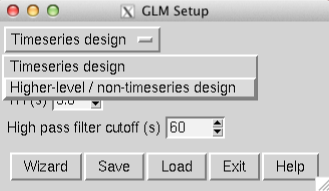
Figure 1: Initial screen of the Glm interface. Change the design type from “Timeseries” to “Higher-level/non-timeseries” and input the number of participants.
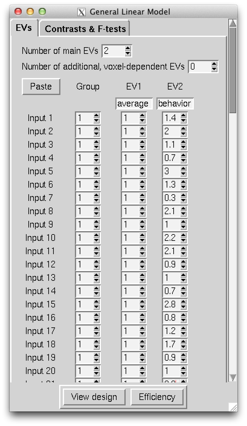
Figure 2: The EVs screen of the Glm interface. This screen is where we enter the independent variables/regressors. In my sample we see two columns, a column of 1s for modelling the group average effect and a column for the individual difference behavior of interest. In this sample I entered z-scores for my behavior of interest. I should note that the paste option comes in handy and allows you to just paste the two columns in from any spdreadsheet program such as Libre Office Calc or Microsoft Excel.
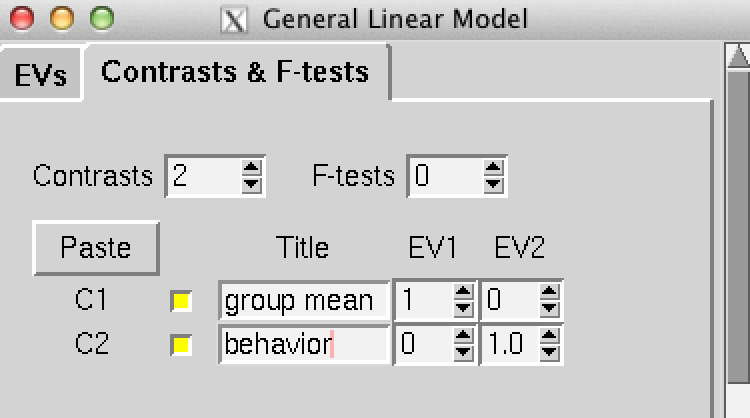
Figure 3: The contrasts screen of the Glm interface. This is a very important screen. We are performing this analysis to model how resting-state networks vary as a function of some individual or group interest. This screen allows us to state what models are run. In my sample above you will see two contrasts, one for modelling the group average and one for modelling the behavioral individual difference. You may want to read the FSL documentation page for the GLM tool to better understand how these contrasts work, but if your design is simple like in this example, you can replicate the screenshot above. It may also be useful to add additional columns for control variabels such as movement in the scanner (e.g., mean translation and/or rotation).
After you finish entering everything, you will want to save you work. In this example, I saved into a “designs” folder. Note that saving creates a design.mat and a design.con file. These are the design matrix and contrasts, respectively.
Running Dual Regression
Running dual regression is very easy. Here is the command I ran for this sample analysis:
$ dual_regression melodic_output.gica/groupmelodic.ica/melodic_IC 1 designs/design.mat designs/design.con 5000 dualreg_output `cat melodic_output.gica/.filelist`
I can break down the various pieces of the command as a suplement to the documentation:
dual_regression: the dual regression command.melodic_output.gica/groupmelodic.ica/melodic_IC: this piece is telling dual regression where to look for the group level ICA components that were generated by Melodic.1: either put a 0 or a 1 here to specify whether or not to variance normalize timecourses during the second stage of the dual regression.designs/design.mat: location of a design matrix file.designs/design.con: location of the design contrasts file.5000: the number of permutations that randomise will run. For publication purposes, people seem to use 5000 or 10000. Note that more permutations = a longer wait.dualreg_output: folder where the output of dual regression will go.cat melodic_output.gica/.filelist: this is a command within a command to list each participant’s preprocessed resting-state scan. Melodic creates this nice list of the files for you, so you can just use the contents of that file rather than having to list them all yourself with a more complicated command.
Visualizing Results
- Identify networks-of-interest
- Determine if there is any behavior-associated variability in these networks
- Plot the results
1. Identify networks-of-interest:
I only care about the contrast of interest (the effect of behavior), so the first thing I do is make a list of the dual regression results that actually matter to me. Another way to reduce the data we need to sort through is to get rid of results for networks that did not significantly correlate with reference networks. In the Melodic guide, we used fslcc to do the reference network correlations. We can pipe that command into a series of other commands and end up with a list of networks to use later as networks of interest:
$ fslcc --noabs -p 3 -t .204 reference_networks/yeo2011_7_liberal_combined.nii.gz melodic_output.gica/groupmelodic.ica/melodic_IC.nii.gz | tr -s ' ' | cut -d ' ' -f 3 | sort -u | awk '{ printf "%02d\n", $1 - 1 }' >> nets_of_interest.txt
That is a lot to look at. The first part is the same correlation command from the Melodic guide. I’ve piped it to tr to clean up fslcc’s terrible white space delimited output. The cut command grabs the third column of numbers from the fslcc output, which corresponds to the network number from the Melodic analysis. sort -u deletes repeat entries (e.g., one network that might have correlated with two seperate reference networks). The awk command adds a 0 to the single digit numbers (e.g., 2 becomes 02) and subtracts 1 from the number because dual regression results start at 0. The whole command is kind of hacky, so feel free to manually compile a list of networks you want to look at in dual regression. If you manually create the list, you also have the opportunity to focus on networks for which you might have a specific a priori hypothesis. I usually generate this list and then delete any for which I am not looking for something specific.
2. Determine if there is any behavior-associated variability in networks-of-interest:
Using the list of networks-of-interest, we can loop through the dual regression results and determine if there are any significant findings. An easy way to figure out if there is any behavior-related variability for a given network is to use the fslstats command to produce the range of p-values in the stat map. Look for stat maps where the range extends past the typical p < 0.05 threshold (so here look for the 1-p range to extend past 0.95).
for i in `cat nets_of_interest.txt`; do
        # Print range of 1-p values to command line:
        echo "The range of 1-p values in image dualreg_output/dr_stage3_ic00${i}_tfce_corrp_tstat2.nii.gz :";
        echo "";
        fslstats dualreg_output/dr_stage3_ic00${i}_tfce_corrp_tstat2.nii.gz -R;
        # Add file location to a text file for creation of PNG images:
        max=`fslstats dualreg_output/dr_stage3_ic00${i}_tfce_corrp_tstat2.nii.gz -R | cut -d " " -f 2`
        thresh="0.9"
        if (( $(echo "$max > $thresh" | bc -l) )); then
            echo "dualreg_output/dr_stage3_ic00${i}_tfce_corrp_tstat2.nii.gz" >> tfce_result_sig.txt;
        fi
    done
This loop also produces a file containing stat maps that contain “significant results” according to a specified p-value. The file is used later to automatically make PNG images of the dual regression results.
3. Plot dual regression results:
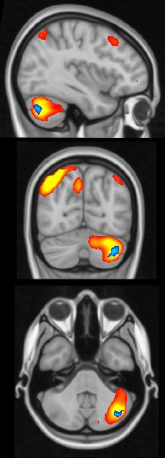
The final step in this analysis is plotting. To view daul regression results from inidividual networks, we can use fslview. The output of dual regression is a stat map that we can overlay on top of the corresponding resting-state network. This command will show areas in blue that are altered in individuals with higher ability in the network of interest (network plotted in warm colors). Remember when adding the melodic component that the thresh_zstat images are numbered starting with 1 while the dual regression output starts with 0. Also, you may need to play with the thresholding.
$ fslview melodic_output/bg_image.nii.gz -l "GreyScale" melodic_output.gica/groupmelodic.ica/stats/thresh_zstat14.nii.gz -l "Red-Yellow" -b 3,12 dualreg_output/dr_stage3_ic0013_tfce_corrp_tstat2.nii.gz -l "Blue-Lightblue" -b .9,1
An optional step would be to automatically generate images of all significant dual regression results on top of the respective resting-state network. Many of the tools within this last script are similar to the ones I use to plot the ICA components in the previous guide, including interpolating a higher resolution stat map and resting-state network. You may need to tweak the slicer command to grab the images from appropriate slices.
behavior="ef" # name of behavior that may correspond to variability in networks
    for i in `cat tfce_result_sig.txt`; do
        file=`echo $i | cut -d "/" -f 2`;
        dualreg_net_num=`echo $i | cut -d "/" -f 2 | cut -d "_" -f 3 | tail -c -3`;
        melodic_net_num=`expr $dualreg_net_num + 1`;
        # render results in higher resolution:
        flirt -in $i -ref $FSLDIR/data/standard/MNI152_T1_0.5mm -applyxfm -usesqform -out presentation/highres_${behavior}_${file};
        # put results on top of network and background brain:
        overlay 1 0 $FSLDIR/data/standard/MNI152_T1_0.5mm -A presentation/thresh_zstat${melodic_net_num}_highres.nii.gz 2.5 10 presentation/highres_${behavior}_${file} .85 1 presentation/highres_${behavior}_overlay_${file};
        # produce png file:
        slicer presentation/highres_${behavior}_overlay_${file} -a presentation/highres_${behavior}_overlay_sliced_dualreg_${dualreg_net_num}.png;
    done
Enjoy the results.